Using KvarQ Graphical User Interface (GUI)
Launching the GUI
Depending on how KvarQ was installed, there are different ways of launching the GUI
- Installation from source: simply enter kvarq gui on the command line or alternatively call python -m kvarq.cli gui. When KvarQ is launched this way, you can use some command line switches (for example specify the directory containing the testsuites).
- Binary installation windows: go to the directory with the KvarQ files and start kvarq-gui.exe
- Binary installation OS X: open the KvarQ application in the Finder
Below is what you should see after launching the GUI
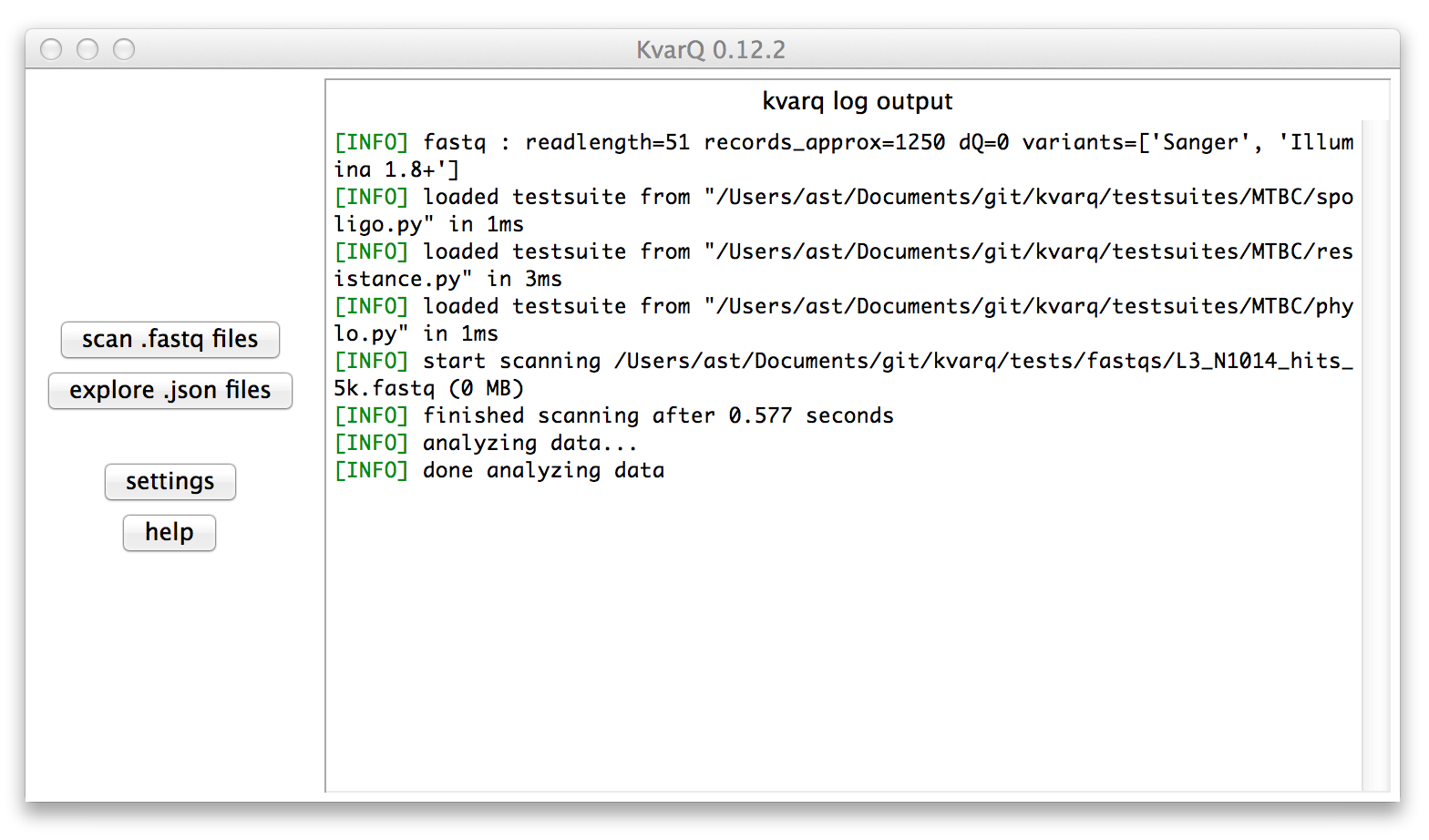
The right pane in the main window shows the log output that describes the general activity as well as useful additional information during the scanning process. Important messages (warnings, errors) are highlighted in red.
The two buttons on the left open the scanner to scan .fastq files and the explorer to view results saved as .json files from previous scans.
Configuring KvarQ
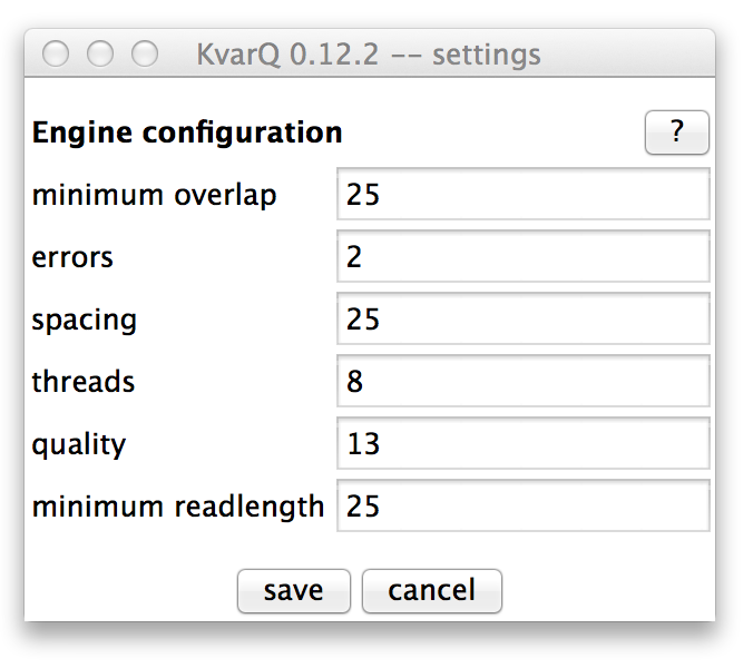
The engine configuration parameters can be modified in the settings window. Usually, the default values work well, but in some cases (such as old low-quality files) it can be advantageous to change some of these values.
The Scanner
This simple window allows to scan a single or multiple .fastq files to generate .json files (depending on whether a single or multiple files are selected in the file selection dialog).
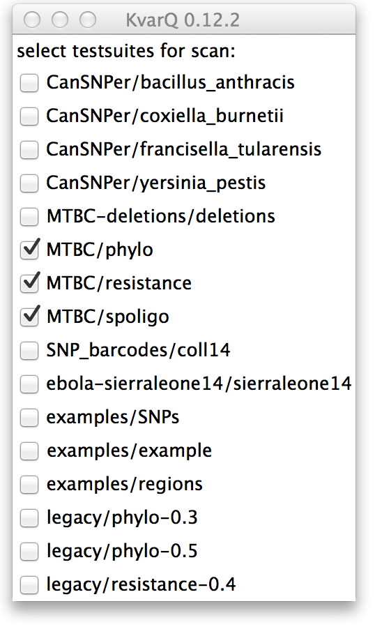
When the selection of .json is done, the scanner shows a window with a list of discovered testsuites that can be checked individually to be included during the scan of the .fastq files.
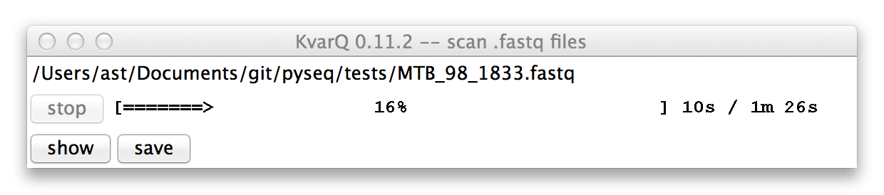
The progress bar (yes, the design is on purpose to remind users to use the command line) shows the progress as well as estimated time left for the current file. The scanning process can be interrupted by clicking on the stop button.
Once the scanning process is done (for all files), the results can be saved to .json files (one per .fastq file). The result of the last scan can also be viewed directly, without saving it to file.
The Explorer
The explorer is a simple Tk program consisting of different windows:
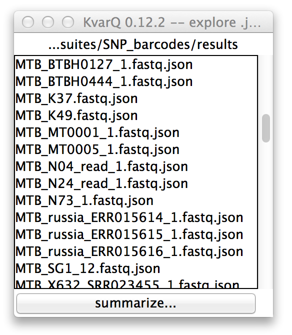
Directory explorer viewing .json files in a directory
Double-clicking any of the list items will open then .json explorer showing details on the selected file.
It is also possible to export the analysis summary of all displayed .json files to a excel sheet by using the button at the bottom of the list.
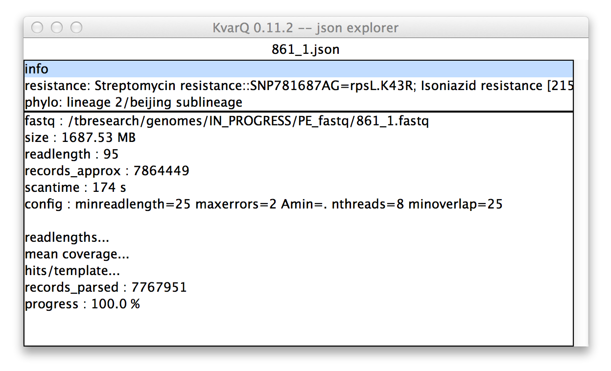
.json explorer showing general information about file
In the upper pane of the .json explorer shows an overview over the file. The contents of the lower pane depend on the selection in the upper pane. Because the info section is selected in the upper pane in this example, the lower pane shows general information about the scanning process, such as the scantime or the kvarq.engine configuration.
The items ending with ... open another window when double-clicked (similar to the coverages described below).
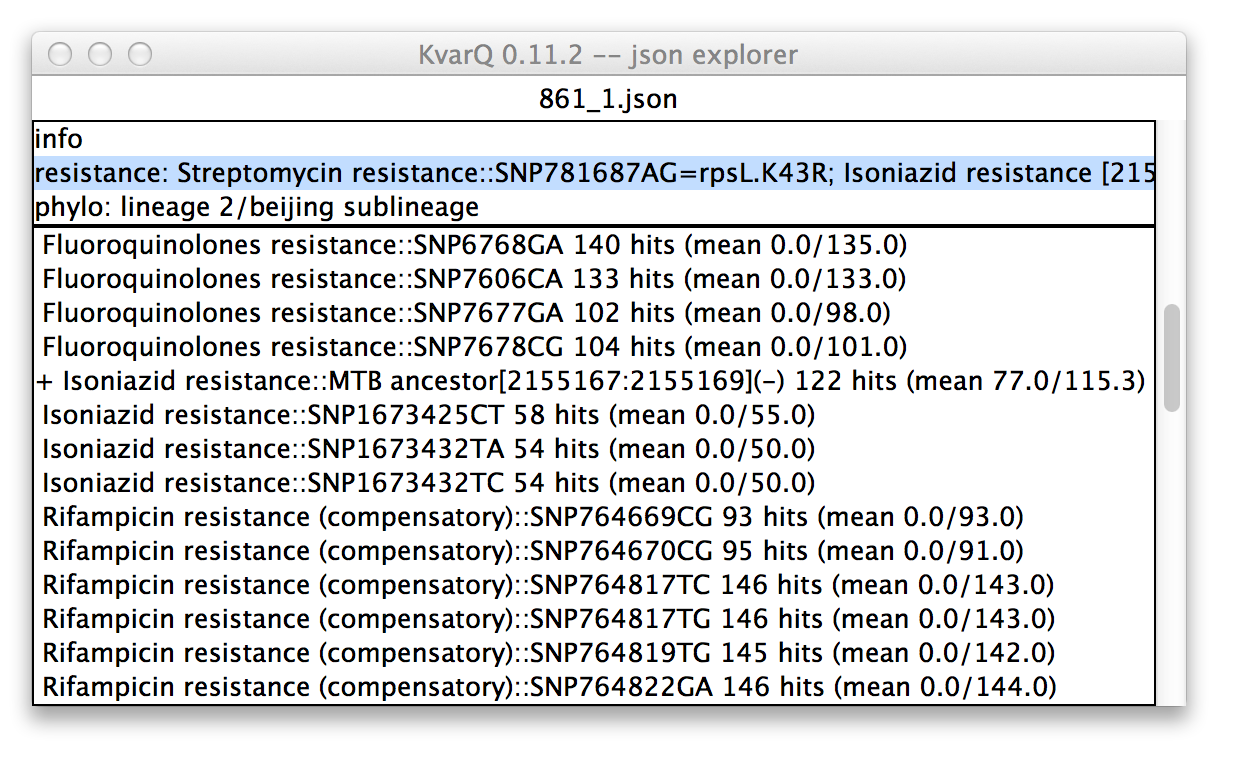
.json explorer showing analysis test details
In this case, the phylogenetic suite was selected in the upper pane. Therefore, all tests belonging to this testsuite are displayed in the lower pane. Every item in the upper pane (apart from the “info” item) consists of the testsuite name (in this case “phylo”) and the summarized result (in this case lineage 2, sublineage bejing).
Every item in the lower pane informs about the following test details:
- Whether the test was “found positive” : a + sign in front of the test name signifies that this test was positive. For a SNP this means that the specified mutant allele was found and for a test covering a larger region of the genome this signifies that there was at least one mutation detected in the region of interest. A ~ sign (not shown) in front of the test name would mean that there were base calls with the most dominant base below 90%, suggesting a mixed colony.
- Test name that describes the genotype.
- Double semicolon :: followed by description of what was tested (this can be a SNP or a region; regions are specified by their start/stop base position and a + or - specifying which strand is coding at this position).
- Double-clicking on an item in the lower pane opens a coverage window.
Interpreting Coverages
KvarQ displays the results of the scanning process in the form of coverages. This display shows information about how many reads were mapped against the sequence of interest and whether there were any mutations detected. The same display is used for SNPs as well as for longer regions, althoug the signification of the displayed elements is somewhat different.
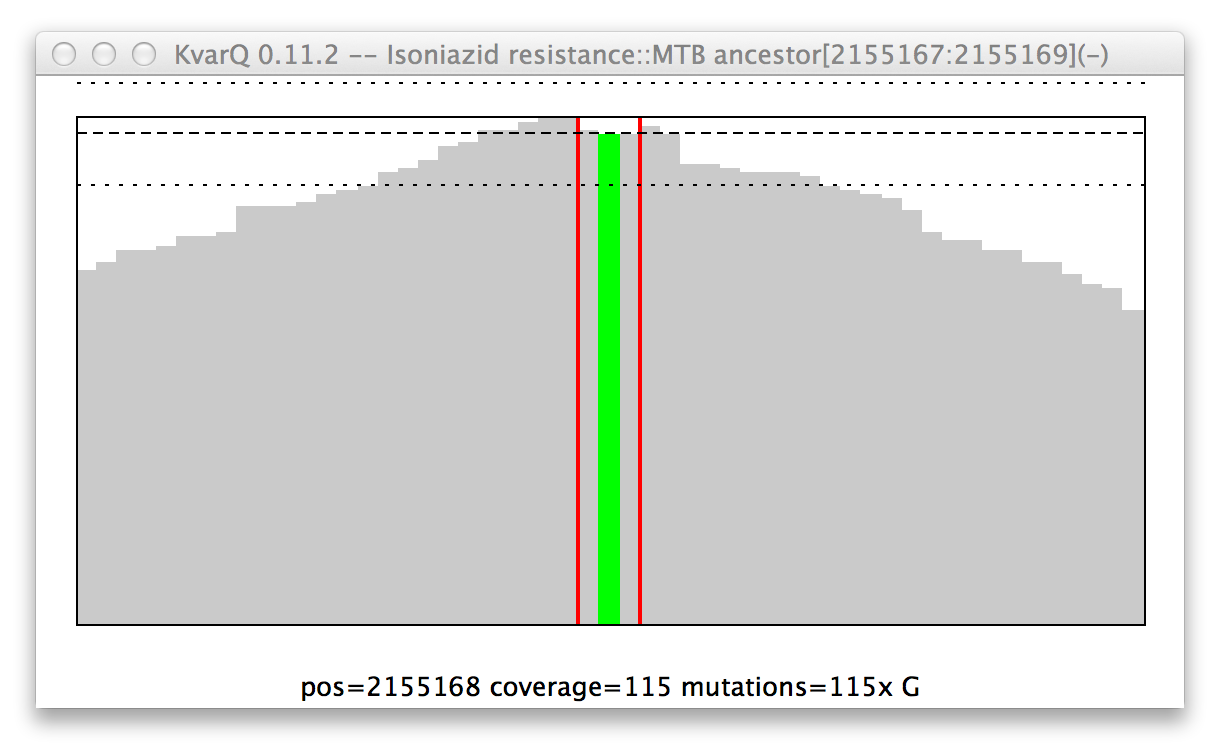
Mutation in the katG resistance confering codon.
General structure of a coverage window:
- The x axis is the genome position. Add the number showed on the x axis to the base position in parantheses in the figure title.
- The y axis is depth of coverage, piling all reads up that mapped to the given positions.
- The red vertical lines show start and stop of the region of interest. In this case, the region of interest is only three bases long, but 25 bases of spacers are added on either side when scanning for the region (see Configuration Parameters).
- The horizontal lines are mean and pseudo-variations of coverage over the region of interest.
- The colored graphs show mutations. In this example there is clearly a mutation that replaced the second base with a guanosine nucleotide. Note that not every read showed this mutation, but a handful had the original base (if every single read showed this mutation, the colored line would go all the way up to the thick black line).
- Moving the mouse over the graph shows quantitative information about the hovered genome position at the bottom of the graph.
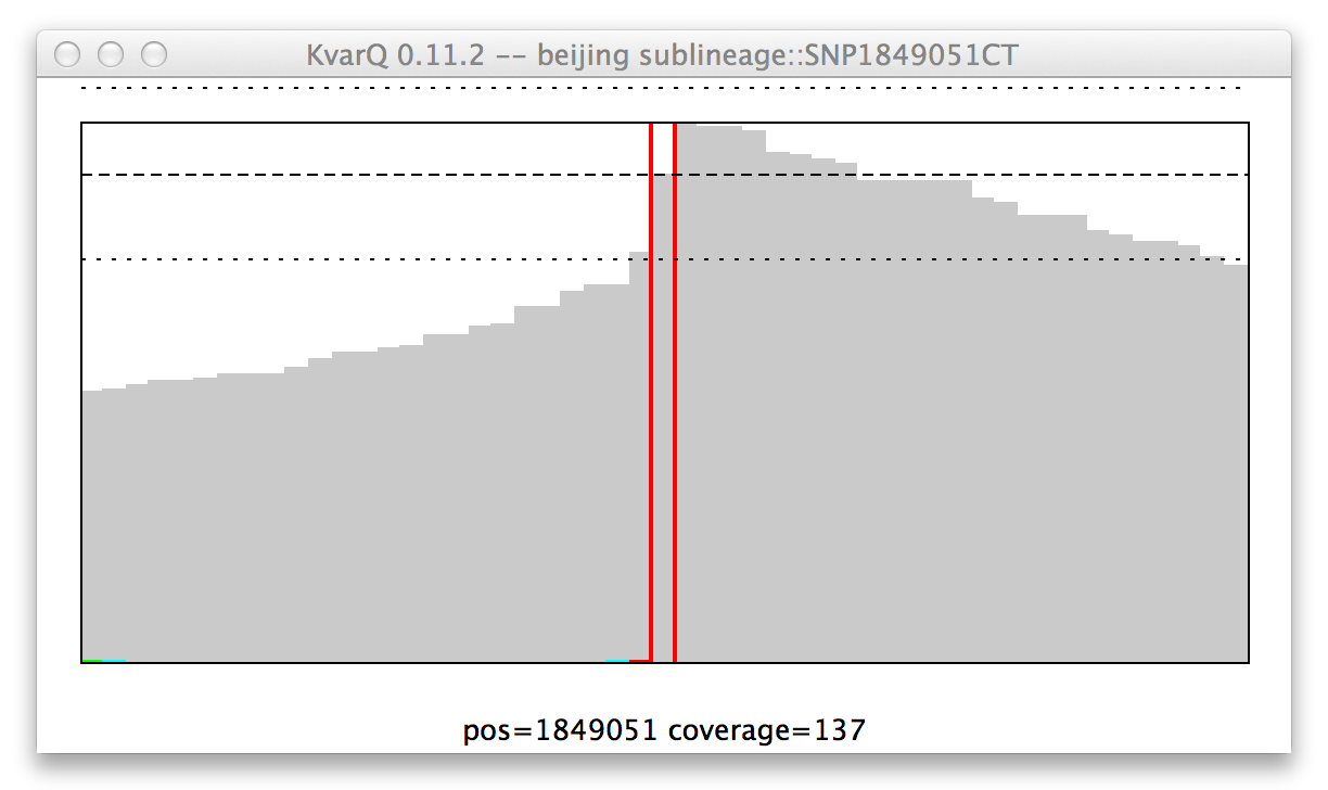
Coverage of a single nucleotide polyphormism (SNP), mutant genotype.
Because KvarQ is looking for a specific mutant sequence, the SNP is “found” if there is no mutation at its position, as is the case in this example (i.e. at position 157129 there is really a T and not a C).
Note: “No color” means mutant for SNP, while it means wild type for regions...
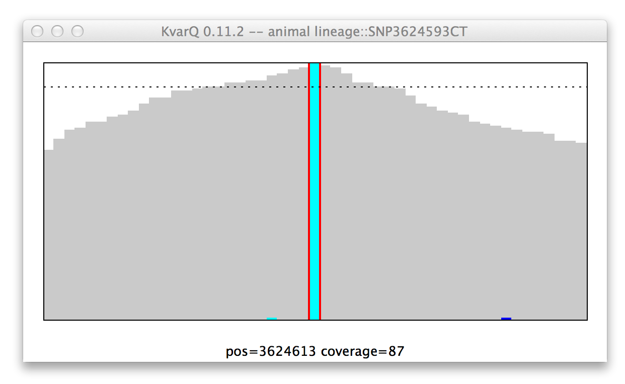
Coverage of a single nucleotide polyphormism (SNP), wildtype genotype.